SPM Machines: A Guide to Voltage and Current Diagram

October 15, 2024

This article aims to explain the circle diagram and its application for surface-mounted permanent magnet (SPM) machines. Before diving into these aspects, it’s necessary to derive the voltage equation for the machine in the dq reference frame in terms of machine inductance, current, speed, and permanent magnet flux linkage. By transitioning from the abc reference frame to the dq reference frame, we obtain two orthogonal components, allowing the creation of the circle diagram.

Voltage Equation in dq reference frame:

Let’s begin with the fundamental voltage equations for the machine, as outlined below.

$v_a=\frac{d}{d t} \lambda_a+i_a r_1$

$v_b=\frac{d}{d t} \lambda_b+i_b r_2$

$v_c=\frac{d}{d t} \lambda_c+i_c r_3$

where $v_a$ , $v_b$ , and $v_c$ are the stator terminal voltages in phases $a$ , $b$ , and $c$ ; $\lambda_a$ , $\lambda_b$ , and $\lambda_c$ are the flux linkages in the abc reference frame; $i_a$ , $i_b$ , and $i_c$ are the abc stator currents; and $r_1$ , $r_2$ , and $r_3$ are the stator resistances for each phase of the stator winding. For simplification and easier discussion, we will neglect the phase resistance in the next step. Thus, we have:

$v_a=\frac{d}{d t} \lambda_a$

$v_b=\frac{d}{d t} \lambda_b$

$v_c=\frac{d}{d t} \lambda_c$

By applying the Park transformation[see the related article for definition and assumptions] and disregarding the zero-sequence component (valid for symmetrical winding and excitation), the dq components of the flux linkages can be expressed as follows:

$\lambda_d= & \frac{2}{3}\left[\lambda_a \cos \left(\theta\right)+\lambda_b \cos \left(\theta-\frac{2 \pi}{3}\right)+\lambda_c \cos \left(\theta+\frac{2 \pi}{3}\right)\right]$

$\lambda_q= & -\frac{2}{3}\left[\lambda_a \sin \left(\theta\right)+\lambda_b \sin \left(\theta-\frac{2 \pi}{3}\right)+\lambda_c \sin \left(\theta+\frac{2 \pi}{3}\right)\right]$

By taking the derivative of $\lambda_d$ with respect to time, we obtain:

$\frac{d \lambda_d}{d t}= & -\frac{2}{3}\left[\lambda_a \sin \left(\theta\right) \frac{d \theta}{d t}+\lambda_b \sin \left(\theta-\frac{2 \pi}{3}\right) \frac{d \theta}{d t}+\lambda_c \sin \left(\theta+\frac{2 \pi}{3}\right) \frac{d \theta}{d t}\right] \ & +$

$\frac{2}{3}\left[\frac{d \lambda_a}{d t} \cos \left(\theta_r\right)+\frac{d \lambda_b}{d t} \cos \left(\theta_r-\frac{2 \pi}{3}\right)+\frac{d \lambda_c}{d t} \cos \left(\theta_r+\frac{2 \pi}{3}\right)\right]$

By rearranging the equation in the first bracket and substituting the derivative terms of flux linkages with voltage values ( $v_a=\frac{d}{d t} \lambda_a$ , $v_b=\frac{d}{d t} \lambda_b$ , $v_c=\frac{d}{d t} \lambda_c$ ) in the second bracket, we obtain:

$\frac{d \lambda_d}{d t}= & -\frac{d \theta}{d t} \frac{2}{3}\left[\lambda_a \sin \left(\theta\right)+\lambda_b \sin \left(\theta-\frac{2 \pi}{3}\right)+\lambda_c \sin \left(\theta+\frac{2 \pi}{3}\right)\right] \ & +$

$\frac{2}{3}\left[v_a \cos \left(\theta\right)+v_b \cos \left(\theta-\frac{2 \pi}{3}\right)+v_c \cos \left(\theta+\frac{2 \pi}{3}\right)\right]$

Now, examining the term in the first bracket (including $2/3$ ), it’s evident that it follows the Park transformation form and is therefore equal to $\lambda_q$ . The same applies to the term in the second bracket (including $2/3$ ), making it equal to $v_d$ . With $\omega= & \frac{d \theta}{d t}$ , the equation above transforms into

$v_d= & \frac{d \lambda_d}{d t}-\omega \lambda_q$

The same approach can be taken to derive $v_q$ , and when it is derived, it is:

$v_q= & \frac{d \lambda_q}{d t}+\omega \lambda_d$

In a steady state within the dq reference frame, both $\lambda_d$ and $\lambda_q$ are constant and therefore their derivatives with respect to time are zero. Hence, we obtain:

$v_d= & -\omega \lambda_q$

$v_q= & +\omega \lambda_d$

Now, let’s express the flux linkage using more easily measurable and calculable machine parameters such as current and inductance, (i.e. $\lambda_d=L_d i_d+\lambda_{pm}$ and $\lambda_q=L_q i_q$ ). Also, in a SPM machine, $L_d=L_q=L_s$ , therefore, $L_d$ and $L_q$ are replaced with $L_s$ which is the synchronous inductance of the machine. Therefore:

$v_d= & -\omega L_s i_q$

$v_q= & \omega L_s i_d + \omega \lambda_{pm}$

where $v_d$ , $v_q$ , $i_d$ and $i_q$ are the d- and q-axis components of the stator voltage and current, respectively, and $V_c$ and $I_c$ are the rated inverter phase voltage and current.

With these basic equations, we can now analyze the circle diagram of a motor-drive system. Drives often have voltage and current ratings ( $V_c$ and $I_c$ , respectively) that limit the machine’s performance before it reaches its thermal limits. These limitations can be expressed by

$\sqrt{{i_d}^2+{i_q}^2}<I_c$

$\sqrt{{v_d}^2+{v_q}^2}<V_c$

Remember that we initially ignored the phase resistance for simplicity. We can continue to ignore it if it is small or if we need an approximate analysis. Alternatively, we could include it by subtracting the voltage drop due to the winding resistance from the rated voltage of the drive. For this discussion, we will continue to ignore it.

Voltage and Current Circle Diagram – Creation:

Both absolute and p.u. values of motor drive parameters can be used to create voltage and current circle diagram. For specific machines and their actual operating conditions, the absolute-value approach is preferred. However, to normalize, compare different machines, and simplify analysis and calculations, the p.u. approach is favored.

To use the p.u. approach, a set of base quantities to normalize system parameters is needed. These base quantities are:

Phase voltage $V_b$ and phase current $I_b$ , equal to their rated values.
Base power $P_b$ , calculated as $P_b=I_b×V_b$ .
Base speed, equal to the rated speed.
Base inductance $L_b$ , given by $L_b= \frac{ V_b}{\omega_b I_b}$ .
Base flux linkage, equal to base torque divided by base current.

This method converts parameters such as voltage, current, power, and inductance into dimensionless values based on the selected base quantities. The below identities show the p.u. values of the related machine parameters.

$V_{pu} \equiv \frac{V}{V_b} \quad I_{pu} \equiv \frac{I}{I_b} \quad \omega_{pu} \equiv \frac{\omega}{\omega_b} \quad L_{pu} \equiv \frac{L}{L_b} \quad \lambda_{pu} \equiv \frac{\lambda}{\lambda_b}$

Transforming the voltage equations (for $v_d$ and $v_q$ ) and the voltage and current limit equations, along with the torque equation for the SPM machine ( $T=\lambda_{pm} i_q)$ ) into their per-unit representations gives:

$v_{d_{pu}}=-\omega_{pu} L_{s_{pu}} i_{q_{pu}}$

$v_{q_{pu}}=\omega_{pu} L_{s_{pu}} i_{d_{pu}} + \omega_{pu} \lambda_{pm_{pu}}$

$T_{pu}}=\lambda_{pm_{pu}} i_{q_{pu}}$

where

$\sqrt{{i_{d_{pu}}}^2+{i_{q_{pu}}}^2}<1$

$\sqrt{{v_{d_{pu}}}^2+{v_{q_{pu}}}^2}<1$

From this point onward, everything is in p.u. Therefore, we’ll omit the $"pu"$ from the subscripts of the machine parameters, assuming all values are in the p.u. system.

The current limit circle can be directly plotted in the $i_d$ $i_q$ plane, encapsulating the feasible operating region.

$\sqrt{{i_d}^2+{i_q}^2}<1$

To plot the voltage limit circle on the same plane, $v_d$ and $v_q$ in $\sqrt{{v_d}^2+{v_q}^2}<1$ need to be rewritten in terms of $i_d$ and $i_q$ . This is achieved by substituting $v_d$ and $v_q$ in the voltage limit equation with the respective $v_d$ and $v_q$ equations in terms of inductance, current and permanent magnet flux linkage.

${(-\omega L_s i_q)}^2+{(\omega L_s i_d + \omega \lambda_{pm})}^2<1$

Now, all terms in the equation are divided by ${(\omega L_s)}^2$ :

${i_q}^2+{(i_d+\frac{\lambda_{pm}}{L_s}})}^2}<\frac{1}{{\omega L_s}}^2$

resulting in a circle equation with its center at $\frac{- \lambda_{pm}}{L_s}$ and a radius of $\frac{1}{\omega L_s}$ .

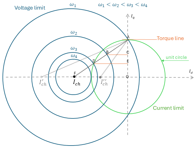
With this, both the current and voltage circles are expressed in terms of $i_d$ and $i_q$ . We can now fully create the diagram. All feasible operating points must lie within both circles. Remember, the green current circle represents a single unit circle. Each blue voltage circle corresponds to a different operating speed, with all circles sharing the same center at $I_{ch}=\frac{- \lambda_{pm}}{L_s}$ . The torque lines, depicted in red, are straight and parallel to the $d-$ axis, proportional to the $i_q$ current.

Voltage and Current Circle Diagram – Application:

With the circle diagram created, we can now explore its insights. This diagram offers a clear geometric representation of the machine’s operation, its limitations, and potential design adjustments to achieve the desired performance.

As mentioned, feasible operating points should fall within both the current and voltage circles. The radius of the voltage circle is inversely proportional to speed, so from zero to rated speed, the radius of voltage circle is large enough to cover all feasible operating point within the current circle. Therefore, in this speed range, the motor drive is limited only by current, which is in this discussion refers to the maximum available drive current. However, there are thermal limits, which are beyond the scope of this discussion.

In this region, the machine can operate with unity current, providing unity torque, meaning it operates at the top of the current limit circle. Hence, the current phase advance is zero (the angle between the current and the $q-$ axis), with $i_q$ equal to the maximum available current and $i_d$ equal to zero. This speed range is known as the constant torque region. The base speed can be geometrically identified here—it is the speed at which the voltage limit circle intersects the current limit circle and unity torque line, denoted by $\omega_1$ in the figure above. At base speed, current, voltage, and torque are all at unity.

As the machine speed exceeds base speed, the voltage limit shrinks from the circle labeled $\omega_1$ (base speed), introducing the voltage limitation into the equation. For example, consider $\omega_2$ . The operating point at each speed is defined by the $i_d$ and $i_q$ values at that speed, which give a certain torque. To achieve maximum torque under these conditions, the current values must fall within both the current and voltage limit circles. Note that the current limit ensures the current remains within the rated current of the machine, while the voltage limit represents the locus of feasible current values from a voltage perspective, considering the effects of current and speed on the terminal voltage to ensure it does not exceed the motor drive voltage limit.

At $\omega_2$ , $i_q$ decreases (from its maximum value at $\omega_1$ ), consequently reducing the generated torque. Introducing $i_d$ current increases the current phase advance from its zero value for speed values up to rated speed.

Another operating region for a permanent magnet synchronous machine is the constant power region, which may or may not exist for an SPM motor. At speeds above base speed, torque decreases, and constant power is only relevant if the rate of torque reduction matches the rate of speed increase. This constant power region can be explained using Thales’ Theorem (basic proportionality theorem) applied to the triangle formed by OAF in the figure above. Point O is the origin, and line AF connects the center of the voltage limit circle to the maximum current value in the $q-$ axis. The aim is to understand how the constant power region is possible and its extent. In the OAF triangle, parallel lines such as BC and DE correspond to speeds $\omega_2$ and $\omega_3$ , respectively. The power at base speed equals $T(\omega_1) \omega_1$ . Applying the basic proportionality theorem to triangle OAF and considering the parallel line BC (corresponding to speed $\omega_2$ ), we have…

$\frac{A B}{B F}=\frac{A C}{C O} \rightarrow \frac{A F}{B F}=\frac{A O}{C O}$

We also know from the voltage limit equation that the radius at any given speed is inversely proportional to the speed. Using this, let’s substitute the values for AF, BF, AO, and CO into the equation $\frac{A F}{B F}=\frac{A O}{C O}$ .

AO represents the rated current (purely $i_q$ ), while CO denotes $i_q$ at the speed $\omega_2$ when the machine is operating along line AF. The length of AF is proportional to the inverse of $\omega_1$ , and BF is proportional to the inverse of $\omega_2$ . Therefore

$\frac{\frac{1}{\omega_1}}{\frac{1}{\omega_2}}=\frac{I q\left(\omega_1\right)}{I q\left(\omega_2\right)}$

Where $i_q(\omega_1)$ and $i_q(\omega_2)$ represent the $i_q$ current at speeds $\omega_1$ and $\omega_2$ respectively, when the operating points lie on the AF line. This means $i_q$ (or torque) decreases at the same rate as speed increases when the machine operates along the AF line, thus generating the same power at $\omega_2$ as it did at $\omega_1$ . Applying the basic proportionality theorem to the OAF triangle with the parallel line DE corresponding to speed $\omega_3$ , we can calculate the same constant power.

This region, spanning from speed $\omega_1$ to $\omega_3$ is known as the constant power region. This is not always guaranteed in SPM machines. Two different scenarios are shown: one with a characteristic current $I''_{ch}$ within the current limit, which results in an infinite constant power region (though this may be impractical due to inherent machine friction), and another with $I'_{ch}$ positioned further left from the current circle, indicating a very limited constant power region. The constant power region may not exist at all.

Increasing the speed beyond $\omega_3$ leads to a rapid reduction in torque, as the constant power line moves outside the current limit circle at that speed. At $\omega_4$ , there are no feasible current values within the current limit that meet the voltage limit, as there is no overlap between the voltage and current circles. Therefore, $\omega_4$ is the maximum speed of the machine.

In summary, the voltage and current diagram provides a geometric representation of the relationships between current, voltage, and speed in an SPM machine, highlighting the limitations of this type of machine.