Exploring Park, Clarke, and Concordia Transformations

October 1, 2024

“The only constant is change.” — Heraclitus

To facilitate the analysis of a three-phase system, mathematical transformations can be utilized to convert the three-phase signals into two orthogonal* components. The Park transformation is the most commonly used method. However, Clarke and Concordia transformations are also examined due to their close relationship. These transformations can initiate the conversion from the abc to the dq reference frame, although this step is not mandatory.

Clarke and Concordia Transformations:

The Clarke and Concordia transformations function within a stationary reference frame, leading to varying transferred components. The Clarke transformation ensures magnitude invariance, while the Concordia transformation maintains power invariance.

\[\left[\begin{array}{l}\alpha \\ \beta \\ 0\end{array}\right]=\frac{2}{3}\left[\begin{array}{ccc}1 & -\frac{1}{2} & -\frac{1}{2} \\ 0 & \frac{\sqrt{3}}{2} & -\frac{\sqrt{3}}{2} \\ \frac{1}{2} & \frac{1}{2} & \frac{1}{2}\end{array}\right]\left[\begin{array}{l}a \\ b \\ c\end{array}\right]\]

\[\left[\begin{array}{l}\alpha \\ \beta \\ 0\end{array}\right]=\sqrt{\frac{2}{3}}\left[\begin{array}{ccc}1 & -\frac{1}{2} & -\frac{1}{2} \\ 0 & \frac{\sqrt{3}}{2} & -\frac{\sqrt{3}}{2} \\ \sqrt{\frac{1}{2}} & \sqrt{\frac{1}{2}} & \sqrt{\frac{1}{2}}\end{array}\right]\left[\begin{array}{l}a \\ b \\ c\end{array}\right]\]

The coefficient before the transformation matrix guarantees that the transformation remains magnitude invariant for the Clarke transformation or power invariant for the Concordia transformation.

The first and second rows of the transformation matrices represent the projection coefficients of the three-phase components onto the alpha and beta axes, respectively.

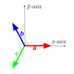
For example, considering two reference frames demonstrated in figure above and with the alpha axis aligned with the a-axis and beta axis leading the alpha axis, the projection of the three-phase components onto the alpha axis is

$f_\alpha=f_a+f_b \cdot \cos \left(240^{\circ}\right)+f_c \cdot \cos \left(120^{\circ}\right)=f_a-\frac{1}{2} f_b-\frac{1}{2} f_c$

where $f_a$ , $f_b$ and $f_c$ are the three-phase components in the abc reference frame, and $f_\alpha$ is in the stationary αβ reference frame. The same logic applies to the second row. Note that the projection angle is measured counterclockwise from the abc components to the alpha-beta axis.

The third row represents the zero-sequence component, which is the average of the three-phase components and can be expressed as $f_0 = \frac{1}{3}(I_a + I_b + I_c)$ . Ignoring the coefficient before the transformation matrix, the third row in the transformation matrix is $\begin{bmatrix}\frac{1}{3} & \frac{1}{3} & \frac{1}{3}\end{bmatrix}$ . To maintain the same zero-sequence component equation, the third row must be adjusted by considering the factor before the matrix in each transformation.

Park Transformation:

Unlike Clarke and Concordia transformations, the Park transformation operates in a rotating reference frame, resulting in constant (or DC) components. This rotating reference frame is stationary relative to the rotor but rotates with respect to the abc reference frame. Therefore, defining the rotor position is necessary. The rotor position is the angle between the rotor’s magnetic axis and the magnetic axis of stator phase A. This angle can align with either the direct axis (d-alignment) or the quadrature axis (q-alignment). By aligning the a-axis of the abc system with either the d-axis or q-axis of the rotating reference frame at time ( t = 0 ), the rotor position is given by $\theta = \omega \cdot t$ .

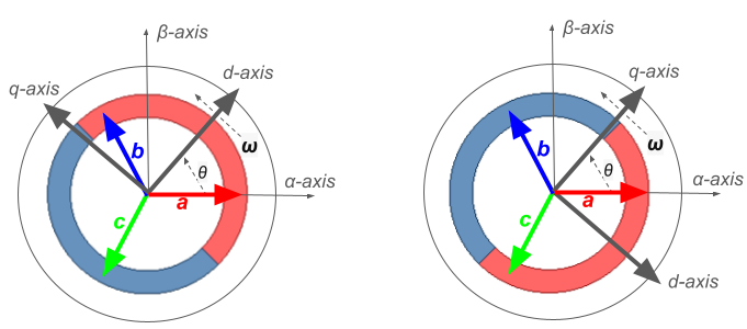
Red pole is north, and blue pole is south.

The same procedure used for the Clarke and Concordia transformations is applied here by projecting the abc components onto the d and q axes, considering the rotor angle. For example, the first row of the transformation matrix for the d-alignment case can be calculated by projecting the abc components onto the d-axis as follows:

$f_d = f_a \cos(\theta) + f_b \cos(240^\circ + \theta) + f_c \cos(120^\circ + \theta)$

In literature, authors use the angle $( \theta - 120^\circ )$ instead of $( 240^\circ + \theta )$ because it is standard notation. The $( 120^\circ )$ phase shift is natural for three-phase systems, making $( \theta - 120^\circ )$ more intuitive for readers familiar with these systems.

The third row relates to the zero-sequence component, which becomes significant when the system encounters conditions that deviate from its normal balanced state, leading to zero-sequence components, or during normal operation when zero-sequence current or voltage is involved.

\[\left[\begin{array}{l}d \\ q \\ 0\end{array}\right]=\frac{2}{3}\left[\begin{array}{ccc}\cos (\theta) & \cos \left(\theta-\frac{2 \pi}{3}\right) & \cos \left(\theta+\frac{2 \pi}{3}\right) \\-\sin (\theta) & -\sin \left(\theta-\frac{2 \pi}{3}\right) & -\sin \left(\theta+\frac{2 \pi}{3}\right) \\ \frac{1}{2} & \frac{1}{2} & \frac{1}{2}\end{array}\right]\left[\begin{array}{l}a \\ b \\ c\end{array}\right]\]

\[\left[\begin{array}{l}d \\ q \\ 0\end{array}\right]=\sqrt{\frac{2}{3}}\left[\begin{array}{ccc}\cos (\theta) & \cos \left(\theta-\frac{2 \pi}{3}\right) & \cos \left(\theta+\frac{2 \pi}{3}\right) \\-\sin (\theta) & -\sin \left(\theta-\frac{2 \pi}{3}\right) & -\sin \left(\theta+\frac{2 \pi}{3}\right) \\ \sqrt{\frac{1}{2}} & \sqrt{\frac{1}{2}} & \sqrt{\frac{1}{2}}\end{array}\right]\left[\begin{array}{l}a \\ b \\ c\end{array}\right]\]

* From a geometric standpoint, the alpha-beta axes in Clarke and Concordia transformations and the d-q axes in the Park transformation are orthogonal. However, the requirement for the transformation to be power-invariant only if the transformation matrix is orthogonal stems from the mathematical definition of orthogonality. For a matrix to be orthogonal, its inverse must equal its transpose, a condition satisfied by the coefficient of $\sqrt{\frac{2}{3}}$ in the Concordia transformation matrix. The same coefficient can be applied to the Park transformation to make it orthogonal and power-invariant.

d-alignment magnitude-invariant	$\left[\begin{array}{l}d \\ q \\ 0\end{array}\right]=\frac{2}{3}\left[\begin{array}{ccc}\cos (\theta) & \cos \left(\theta-\frac{2 \pi}{3}\right) & \cos \left(\theta+\frac{2 \pi}{3}\right) \\-\sin (\theta) & -\sin \left(\theta-\frac{2 \pi}{3}\right) & -\sin \left(\theta+\frac{2 \pi}{3}\right) \\ \frac{1}{2} & \frac{1}{2} & \frac{1}{2}\end{array}\right]\left[\begin{array}{l}a \\ b \\ c\end{array}\right]$
d-alignment power-invariant	$\left[\begin{array}{l}d \\ q \\ 0\end{array}\right]=\sqrt{\frac{2}{3}}\left[\begin{array}{ccc}\cos (\theta) & \cos \left(\theta-\frac{2 \pi}{3}\right) & \cos \left(\theta+\frac{2 \pi}{3}\right) \\-\sin (\theta) & -\sin \left(\theta-\frac{2 \pi}{3}\right) & -\sin \left(\theta+\frac{2 \pi}{3}\right) \\ \sqrt{\frac{1}{2}} & \sqrt{\frac{1}{2}} & \sqrt{\frac{1}{2}}\end{array}\right]\left[\begin{array}{l}a \\ b \\ c\end{array}\right]$
q-alignment magnitude-invariant	$\left[\begin{array}{l}d \\ q \\ 0\end{array}\right]=\frac{2}{3}\left[\begin{array}{ccc}\sin(\theta) & \sin\left(\theta-\frac{2 \pi}{3}\right) & \sin\left(\theta+\frac{2 \pi}{3}\right) \\\cos(\theta) & \cos\left(\theta-\frac{2 \pi}{3}\right) & \cos\left(\theta+\frac{2 \pi}{3}\right) \\ \frac{1}{2} & \frac{1}{2} & \frac{1}{2}\end{array}\right]\left[\begin{array}{l}a \\ b \\ c\end{array}\right]$
q-alignment power-invariant	$\left[\begin{array}{l}d \\ q \\ 0\end{array}\right]=\sqrt{\frac{2}{3}}\left[\begin{array}{ccc}\sin(\theta) & \sin\left(\theta-\frac{2 \pi}{3}\right) & \sin\left(\theta+\frac{2 \pi}{3}\right) \\\cos(\theta) & \cos\left(\theta-\frac{2 \pi}{3}\right) & \cos\left(\theta+\frac{2 \pi}{3}\right) \\ \sqrt{\frac{1}{2}} & \sqrt{\frac{1}{2}} & \sqrt{\frac{1}{2}}\end{array}\right]\left[\begin{array}{l}a \\ b \\ c\end{array}\right]$

Clarke transformation	$\left[\begin{array}{l}\alpha \\ \beta \\ 0\end{array}\right]=\frac{2}{3}\left[\begin{array}{ccc}1 & -\frac{1}{2} & -\frac{1}{2} \\ 0 & \frac{\sqrt{3}}{2} & -\frac{\sqrt{3}}{2} \\ \frac{1}{2} & \frac{1}{2} & \frac{1}{2}\end{array}\right]\left[\begin{array}{l}a \\ b \\ c\end{array}\right]$
Concordia transformation	$\left[\begin{array}{l}\alpha \\ \beta \\ 0\end{array}\right]=\sqrt{\frac{2}{3}}\left[\begin{array}{ccc}1 & -\frac{1}{2} & -\frac{1}{2} \\ 0 & \frac{\sqrt{3}}{2} & -\frac{\sqrt{3}}{2} \\ \sqrt{\frac{1}{2}} & \sqrt{\frac{1}{2}} & \sqrt{\frac{1}{2}}\end{array}\right]\left[\begin{array}{l}a \\ b \\ c\end{array}\right]$